


NumPy (short for Numerical Python) is a Python library for scientific computing that provides support for arrays and matrices, along with a large number of mathematical functions to operate on them. It also forms the base of python library Pandas. In this blog, I will try to explain all the different numpy functions and concepts that will more than cover your basics of numpy. So, if you are a beginner, this blog is for you.
Python List vs Numpy Array
Python lists and numpy arrays are both used to store and manipulate data, but they have some key differences in terms of functionality and performance.
- Functionality:
Python lists are flexible and can store data of any type, including strings, numbers, and other objects. Lists are also mutable, which means you can add, remove, or change elements in a list after it has been created.
On the other hand, numpy arrays are homogeneous, meaning they can only store elements of the same type. However, numpy arrays provide a wide range of mathematical and statistical functions, making it easy to perform operations on arrays, such as matrix multiplication, dot product, and statistical analysis.
- Performance:
Numpy arrays are faster than Python lists for numerical operations because they are implemented in C and use contiguous blocks of memory, which allows for more efficient memory access. In contrast, Python lists are implemented in Python, and they use pointers to reference elements scattered throughout memory, which can slow down operations.
Installing
You can install Numpy by typing the following command in terminal
pip install numpy
After installing you can check the version using
pip show numpy
If installed correctly, it would show something like this
Name: numpy
Version: 1.23.5
Summary: NumPy is the fundamental package for array computing with Python.
Home-page: https://www.numpy.org
Author: Travis E. Oliphant et al.
Author-email:
License: BSD
Location: /Users/pranjalchaubey/anaconda3/lib/python3.10/site-packages
Requires:
Required-by: astropy, bokeh, Bottleneck, contourpy, datashader, datashape, gensim, h5py, holoviews, hvplot, imagecodecs, imageio, imbalanced-learn, matplotlib, numba, numexpr, pandas, patsy, pyerfa, PyWavelets, scikit-image, scikit-learn, scipy, seaborn, statsmodels, tables, tifffile, transformers, xarray
Importing
To use numpy and its functions in your code import it like this
import numpy as np
Creating NumPy array
You can create a numpy array by using the function np.array().
np.array(object, dtype=None, *, copy=True, order='K', subok=False, ndmin=0,like=None)
For example, by passing a list to the function, we can create an array
import numpy as np
a = np.array([1,2,3,4,5])
print(a)
or
import numpy as np
li = [10,20,30]
a = np.array(li)
print(a)
itemsize => lists the size (in bytes) of each array element
nbytes => which lists the total size (in bytes) of the array
To know properties/attributes of ndarray
ndarray.ndim => to know the dimension of the ndarray.
ndarray.dtype => to know the data type of the elements in the ndarray
ndarray.size => to know the total number of elements in the array.
ndarray.shape => returns the shape of an array in tuple form.
ndarray.itemsize => lists the size (in bytes) of each array element.
ndarray.nbytes => which lists the total size (in bytes) of the array.
a = np.array([1,2,3,4,5])
print("The dimensions of the array a:",a.ndim)
print("The data type of elements of array a:", a.dtype)
print("The size of the array a:",a.size)
print("The shape of the array a:",a.shape)
print("itemsize:", x3.itemsize, "bytes")
print("nbytes:", x3.nbytes, "bytes")

#output -
#The dimensions of the array a => 1
#The data type of elements of array a => int32
#The size of the array a => 3
#The shape of the array a => (3,)
#itemsize: 4 bytes
#nbytes: 96 bytes
creation of 2D array --> list of list --> nested list
a = np.array([[10,20,30],[40,50,60],[70,80,90]])
print(type(a))
print(a.ndim)
print(a.dtype)
print(a)
print(a.shape)#(no of rows,no of columns)
print(a.size)# total no of elements
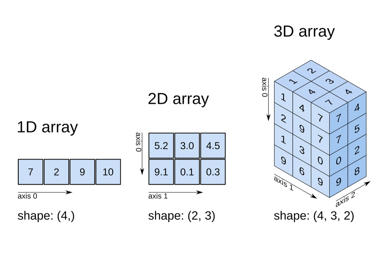
N-dimensional array (ndarray)
A 1D array is a vector while a 2D array is a matrix. Its shape is (number of rows, number of columns).
N-dimension array have axes. 2d array has two axes - axis 0(vertically downward) and axis 1(horizontally across). Similarly, 3d arrays have three axes- axis 0, axis 1 and axis 2.
You can create a 2d numpy array by passing nested lists to np.array function
a = np.array([[10,20,30],[40,50,60],[70,80,90]])
print(type(a))
print(a.ndim)
print(a.dtype)
print(a)
print(a.shape)#(no of rows,no of columns)
print(a.size)# total no of elements

#output -
#<class 'numpy.ndarray'>
#2
#int32
#[[10 20 30]
#[40 50 60]
#[70 80 90]]
#(3, 3)
#9
Note: Unlike Python lists, NumPy is constrained to arrays containing the same type. If types do not match, NumPy will upcast if possible.
Example -
np.array([3.14, 4, 2, 3])
#output -
# array([3.14, 4. , 2. , 3. ])
# here it upcasted integers to float datatype
#If we want to explicitly set the data type of the resulting array, we can use the dtype keyword:
np.array([1, 2, 3, 4], dtype='float')
If we want to explicitly set the data type of the resulting array, we can use the dtype keyword:
np.array([1, 2, 3, 4], dtype='float')
#output - array([1., 2., 3., 4.])

np.array([1, 2, 3, 4,0], dtype='bool')# zero is false and non zero is true
#output - array([ True, True, True, True, False])

np.array([1, 2, 3, 4,0], dtype='complex')
#output - array([1.+0.j, 2.+0.j, 3.+0.j, 4.+0.j, 0.+0.j])

np.array([10,'xyz',20.5,False,1+2j],dtype='object')
#output - array([10, 'xyz', 20.5, False, (1+2j)], dtype=object)

np.array([10,'xyz',20.5,False,1+2j])#all elements will be converted to str type
#output - array(['10', 'xyz', '20.5', 'False', '(1+2j)'], dtype='<U64')
We will learn about all the other data types in numpy later on.
arange()
Returns evenly spaced values with a given interval. It can be used only to create 1D arrays but later on, we will learn about reshape() which can be used to work around this problem.
arange([start,] stop[, step,], dtype=None, *, like=None)

#start : integer or real, optional
#stop : integer or real
#step : integer or real, optional
Some examples of its use
a = np.arange(10)#np.arange(stop)
print(a)
#output - [0 1 2 3 4 5 6 7 8 9]
a = np.arange(1,11)#np.arange(start,stop)
print(a)
#output - [1 2 3 4 5 6 7 8 9 10]
a=np.arange(1,11,2)#np.arange(start,stop,step)
print(a)
#output - [1 3 5 7 9]
a=np.arange(1,11,2,dtype='float')
#output - [1. 3. 5. 7. 9.]
reshape()
Reshaping means changing the shape of an array i.e changing number of rows and columns. You can use reshape() to reshape your array.
Note: While reshaping an array, the number of elements in the original array should match the shape of the new array. For example, if the number of elements in the original array is 9 then the array can be reshaped only into (3,3) array.
Using arange and reshape function together is one the easiest ways to create a basic ndarray.
numpy.reshape(array, newshape, order='C')
Example of its use -
a = np.array([[2,3,4],[11,12,13]])
np.reshape(a,(3,2))
#output - array([[2, 3],
#                [4, 11],
#                [12, 13]])

np.arange(0,9).reshape(3,3)
#output - array([[0, 1, 2],
#                [3, 4, 5],
#                [6, 7, 8]])
we can also reshape using unknown dimensions by passing -1. This means that we want numpy to determine the shape based on number of elements.
np.arange(9).reshape(3,-1)

#output - array([[0, 1, 2],
#                [3, 4, 5],
#                [6, 7, 8]])
#Here -1 means we want numpy to determine dimension based on number of elements.
Other ways to create a numpy array -
linspace()
Return evenly spaced numbers over a specified interval. It can only generate a 1D array. Need to use reshape to make arrays with more dimensions.
linspace(start, stop, num=50, endpoint=True, retstep=False, dtype=None, axis=0)

#start -  The starting value of the sequence.
#stop - The end value of the sequence, unless `endpoint` is set to False.
#num - Number of samples to generate. Default is 50.
#endpoint - If True, `stop` is the last sample. Otherwise, it is not #included.
Some example uses of this function-
np.linspace(0,1,4)
#output - array([0. , 0.33333333, 0.66666667, 1. ])

np.linspace(0,1)# default of num is 50 so we will get 50 values between 0 and 1
#output - array([0. , 0.02040816, 0.04081633, 0.06122449, 0.08163265,
 #0.10204082, 0.12244898, 0.14285714, 0.16326531, 0.18367347,
 #0.20408163, 0.2244898 , 0.24489796, 0.26530612, 0.28571429,
 #0.30612245, 0.32653061, 0.34693878, 0.36734694, 0.3877551 ,
 #0.40816327, 0.42857143, 0.44897959, 0.46938776, 0.48979592,
 #0.51020408, 0.53061224, 0.55102041, 0.57142857, 0.59183673,
 #0.6122449 , 0.63265306, 0.65306122, 0.67346939, 0.69387755,
 #0.71428571, 0.73469388, 0.75510204, 0.7755102 , 0.79591837,
 #0.81632653, 0.83673469, 0.85714286, 0.87755102, 0.89795918,
 #0.91836735, 0.93877551, 0.95918367, 0.97959184, 1. ])

np.linspace(1,100,10,dtype='int')
#output - array([ 1, 12, 23, 34, 45, 56, 67, 78, 89, 100])

np.linspace(0,1,4,endpoint=False,retstep=True)
#output - (array([0. , 0.25, 0.5 , 0.75]), 0.25)

np.linspace(0,10,9).reshape(3,3)
#output - array([[ 0.    1.25  2.5 ]
#                [ 3.75  5.    6.25]
#                [ 7.5   8.75 10.  ]])
zeros()
Return a new array of given shape and type, filled with zeros. It takes shape of array as argument.
zeros(shape, dtype=float, order='C', *, like=None)
Examples of its use
np.zeros(4)#1D array with zeros
#output - array([0., 0., 0., 0.])
np.zeros((5,2))#2D array
#output - array([[0., 0.],
 #               [0., 0.],
 #               [0., 0.],
 #               [0., 0.],
 #               [0., 0.]])
np.zeros((2,3,4),dtype='int')# 3D array
#output - array([[[0, 0, 0, 0],
 #                [0, 0, 0, 0],
 #                [0, 0, 0, 0]],
 #               [[0, 0, 0, 0],
 #                [0, 0, 0, 0],
 #                [0, 0, 0, 0]]])
ones()
exactly the same as zeros except the array is filled with 1. Return a new array of given shape and type, filled with ones.
ones(shape, dtype=None, order='C', *, like=None)
Examples -
np.ones(5)
#output - array([1., 1., 1., 1., 1.])
np.ones(5, dtype = int)
#output - array([1, 1, 1, 1, 1])
np.ones((3, 4))
#output - array([[1., 1., 1., 1.],
#                [1., 1., 1., 1.],
#                [1., 1., 1., 1.]])
fill()
Return a new array of given shape and type, filled with fill_value.
full(shape, fill_value, dtype=None, order='C', *, like=None)
np.full(10,fill_value=2)
#output - array([2, 2, 2, 2, 2, 2, 2, 2, 2, 2])

# 2-D array
np.full((2,3),fill_value=3)
#output - array([[3, 3, 3],
#                [3, 3, 3]])
np.full((2,3,4),8)
#output - array([[[8, 8, 8, 8],
#                 [8, 8, 8, 8],
#                 [8, 8, 8, 8]],
#                [[8, 8, 8, 8],
#                 [8, 8, 8, 8],
#                 [8, 8, 8, 8]]])
eye()
To generate an identity matrix. Return a 2-D array with ones on the diagonal and zeros elsewhere.
eye(N, M=None, k=0, dtype, order='C', *, like=None)
# N: number of rows
# M: number of columns
# k: Index of the diagonal. 0 (the default) refers to the main diagonal.
Example
np.eye(3) #default value of M is None that is no of columns = no of rows
#output - array([[1., 0., 0.],
#                [0., 1., 0.],
#                [0., 0., 1.]])
np.eye(2,3)
#output - array([[1., 0., 0.],
#               [0., 1., 0.]])
np.eye(5,k=1)
#output - array([[0., 1., 0., 0., 0.],
#                [0., 0., 1., 0., 0.],
#                [0., 0., 0., 1., 0.],
#                [0., 0., 0., 0., 1.],
#                [0., 0., 0., 0., 0.]])
np.eye(5,k=-2)
#output - array([[0., 0., 0., 0., 0.],
#                [0., 0., 0., 0., 0.],
#                [1., 0., 0., 0., 0.],
#                [0., 1., 0., 0., 0.],
#                [0., 0., 1., 0., 0.]])
Note: It will returns always 2-D arrays. The number of rows and the number of columns need not be same.
identity()
Return the identity array. exactly same as 'eye()' function except
It is always a square matrix(The number of rows and number of columns are always the same)
only the main diagonal contains 1s'.
identity(n, dtype=None, *, like=None)

#n:  Number of rows (and columns) in `n` x `n` output.
Example
np.identity(5,dtype='int')
#output - array([[1, 0, 0, 0, 0],
#                [0, 1, 0, 0, 0],
#                [0, 0, 1, 0, 0],
#                [0, 0, 0, 1, 0],
#                [0, 0, 0, 0, 1]])
empty()
Return a new array of given shape and type, without initializing entries.
 empty(shape, dtype=float, order='C', *, like=None)

#Examples -
np.empty((3,3))
#output - array([[0.00000000e+000, 0.00000000e+000, 0.00000000e+000],
#                [0.00000000e+000, 0.00000000e+000, 9.07104526e-321],
#                [8.45603440e-307, 4.45046007e-307, 2.37667058e-312]])
np.empty((3,2))
#output - array([[4.24399158e-314, 6.36598738e-314],
#                [4.94065646e-324, 1.69759663e-313],
#                [1.06099790e-313, 6.36598738e-314]])
Here, the output array is filled with junk values.
Generating random numbers
The random module in numpy provides several functions that can be used to generate pseudo-random numbers(integers, floating point) between an interval, of some distribution(Normal, Uniform) and create a numpy array of them.
randint()
To generate random int values in the given range. Return random integers from low (inclusive) to high (exclusive)
randint(low, high=None, size=None, dtype=int)
Example of its use
np.random.randint(10,20)#it will generate only one random value [10,20)
#output - 10

np.random.randint(1,9,size=10)# create a 1D array of size 10 with random values from 1 to 8
#output - array([8, 3, 1, 4, 4, 6, 6, 6, 4, 8])

np.random.randint(100,size=(3,5))#create a 2d array with shape(3,5)--> 15 values from 0 to 99
#output - array([[46, 94, 49, 2, 42],
#               [13, 66, 41, 59, 45],
#               [86, 96, 20, 93, 44]])

a=np.random.randint(1,11,size=(20,30),dtype='int8')
#output - array([[ 6,  6,  1],
#                [10,  8,  2]], dtype=int8)
rand()
Random values in a given shape. Create an array of the given shape and populate it with random samples from a uniform distribution over [0, 1).
 rand(d0, d1, ..., dn)

#d0, d1, ....,dn - The dimensions of the returned array, must be non-negative. Default value is 1.
Example of its use
np.random.rand()#returns a single float value in the range [0,1)
#output - 0.6888155719100035

np.random.rand(10)#create 1d array
#output - array([0.77574398, 0.81681253, 0.59201791, 0.9945461 , 0.33840836,0.86933923, 0.59321542, 0.8556918 , 0.9847741 , 0.41750667])

np.random.rand(3,5)#2d array --> specify only dimension
#output -
#array([[0.71587254, 0.98857878, 0.82162883, 0.36661476, 0.83578959],
#       [0.01365075, 0.40513511, 0.77912904, 0.35856739, 0.35470171],
#       [0.51483683, 0.13313262, 0.82300309, 0.7914927 , 0.40473445]])
uniform()
Draw samples from a uniform distribution.
Samples are uniformly distributed over the half-open interval [low, high) (includes low, but excludes high). In other words, any value within the given interval is equally likely to be drawn by uniform.
uniform(low=0.0, high=1.0, size=None)
Difference between uniform and rand? We can not customize the range in rand() but can do this in uniform().
Examples -
np.random.uniform()# acts as rand()
#output - 0.6709778040900857

np.random.uniform(10,20)
#output - 14.888221004597177

np.random.uniform(10,20,size=10) # 1D array with size 10
#output - array([12.31272924, 13.8902264 , 18.2447736 , 13.64484743, 17.0684421, 12.91598594, 15.37299009, 16.62726592, 17.98248403, 14.3627703 ])
np.random.uniform(10,20,size=(3,5))
#output -
#array([[10.91176622, 17.90365534, 17.57626927,11.22780399,10.7187106],
#[18.78131331, 17.1433094 , 10.19030305, 11.11399179, 17.39759648],
#[16.07031312, 18.55599076, 13.91447705, 17.23264199, 17.04573937]])
randn()
Return a sample (or samples) from the "standard normal" distribution. Creates an array of given shape with values from a normal distribution with mean 0 and variance 1.
 randn(d0, d1, ..., dn)
#d0, d1, ..., dn - dimension of the array
Some examples showing its use
np.random.randn()
#output - 0.8124660306980721
np.random.randn(10)
#output - array([ 1.31494894, 0.9804594 , -0.81068158, 0.74029372, 0.00266866,-1.17542247, 0.93841572, -0.45424196, 1.33136071, 2.33567489])
np.random.randn(2,3)
#output - array([[ 0.05574285, -1.34499108, -0.68054094],
#                [ 1.03116923, -0.13104558, 0.06508116]])
normal()
create an array of given shape and fills it with random values from a normal (Gaussian) distribution.
normal(loc=0.0, scale=1.0, size=None)

#loc -  Mean ("centre") of the distribution.
#scale - Standard deviation (spread or "width") of the distribution.
#size - size of the result array
Here are some examples
np.random.normal()
#output - 0.27746639696617165

np.random.normal(10,4,size=10)
#output - array([12.31138936, 11.34233603, 5.70229283, 8.50380622, 8.0056985 ,9.07191558, 21.19619948, 12.16866835, 7.50107813, 8.22964724])

np.random.normal(10,4,size=(2,2))
#output - array([[10.78955429,  7.11856016],
#                [ 8.01600573, 12.7863051 ]])
Difference between randn() and normal()? randn() gives values from a standard normal distribution with mean 0 and variance 1 while with the normal() function, you can specify the mean and variance of the distribution.
shuffle()
Modify a sequence in place by shuffling its contents. This function only shuffles the array along the first axis of a multi-dimensional array. The order of sub-arrays is changed but their contents remain the same.
shuffle(x)
# x - ndarray or MutableSequence. The array, list or mutable sequence to be shuffled.
Examples -
a=np.arange(9)# [0, 1, 2, 3, 4, 5, 6, 7, 8]
np.random.shuffle(a)# it will not return anything but inline shuffling will happen internally
print(a)
#output - [0, 6, 5, 4, 7, 8, 3, 1, 2]

a=np.random.randint(1,101,size=(3,3))
print(a)
#output - [[23 56 59]
#          [90 99 82]
#          [22 28 80]]
np.random.shuffle(a)
print(a)#order of rows is changed but the contents remain same
#output - [[90 99 82]
#          [22 28 80]
#          [23 56 59]]
Data types of NumPy
If you are following a book or any tutorial on Numpy, chances are they might have been introduced to the NumPy data types much before than I am doing it here. But, I think that it was first necessary to get our hands dirty with some code before learning about all the variety of data types in detail because chances are if you are learning numpy, you are already familiar with what data types are.
NumPy has multiple data types available for use. These are mainly the data types present in python and c
Python data types: int, float, complex, bool and str
Numpy data types: Multiple data types present (Python + C)
i ==> integer(int8,int16,int32,int64)
b ==> boolean
u ==> unsigned integer(uint8,uint16,uint32,uint64)
f ==> float(float16,float32,float64)
c ==> complex(complex64,complex128)
s ==> String
U ==> Unicode String
M ==> datetime etc
int8 ==> i1 ; int16 ==> i2; int32 ==> i4(default)
float16 ==> f2 ; float32 ==> f4(default) ; float64 ==> f8
astype()
this function is used to change the data type of an existing array. It creates a copy of the array with the specified type.
ndarray.astype(dtype)
Some examples-
a = np.array([10,20,30,40])
b = a.astype('float64')
print(f"datatype of elements of array a : {a.dtype}")
print(f"datatype of elements of array b : {b.dtype}")
print(a)
print(b)
#output -
#datatype of elements of array a : int32
#datatype of elements of array b : float64
#[10 20 30 40]
#[10. 20. 30. 40.]
Accessing Elements of array
Different ways to access different elements of a numpy array are -
Indexing
Slicing
Advanced Indexing
Condition Based Selection
Indexing
Like normal arrays or lists, numpy arrays also have indices mapped to the values inside. The index ranges from 0 to n-1 where n is the number of elements in that axis of the array. NumPy supports both +ve and -ve indexing.
1D array
Syntax:
array[index]
Examples -
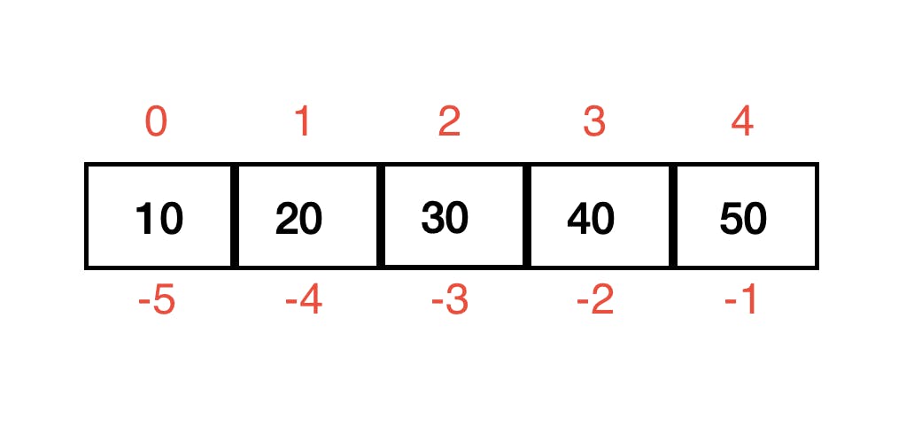
a = np.array([10,20,30,40,50])
a[3]
#output - 40
a[-2]
#output - 40
2D array
Collection of 1-D arrays. There are 2 axes present in the 2-D array -
axis 0: row index
axis 1: column index
Syntax:
array[row_index][column_index]
Example -
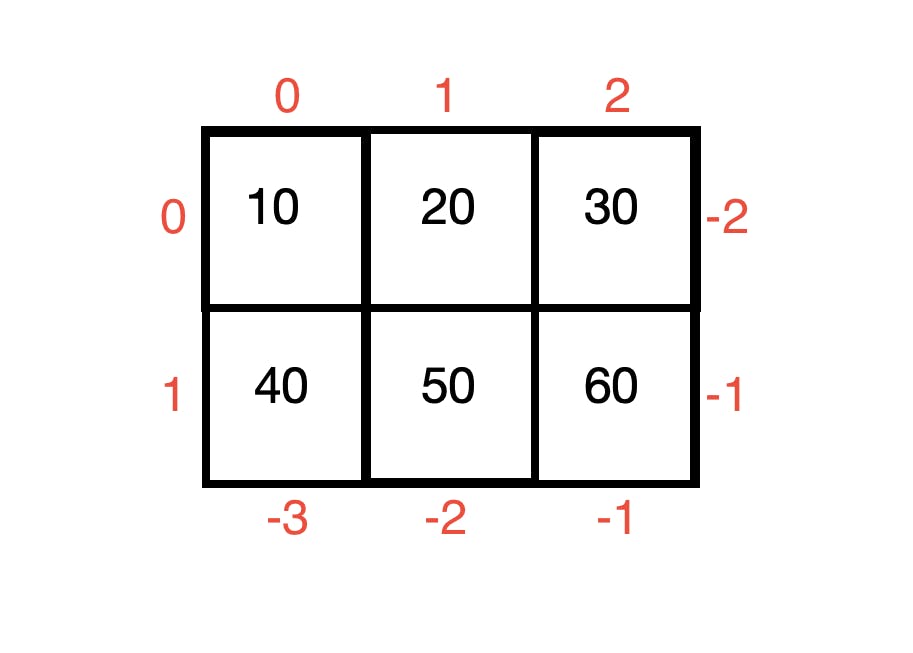
a = np.array([[10,20,30],[40,50,60]])
print(f"Shape of the array a : {a.shape}")
print("To Access the element 50")
print(f"a[1][1] ==> {a[1][1]}")
print(f"a[1][-2] ==> {a[1][-2]}")
print(f"a[-1][2] ==> {a[-1][-2]}")
print(f"a[-1][1] ==> {a[-1][1]}")
#output -
#Shape of the array a : (2, 3)
#To Access the element 50
#a[1][1] ==> 50
#a[1][-2] ==> 50
#a[-1][2] ==> 50
#a[-1][1] ==> 50
Slicing
Used to access multiple elements in some order. Slicing a numpy array is really similar to slicing a python list.
Syntax: array_name[begin:end:step]
#begin(optional): default value is 0
#end: exclusive
#step(optional): default value is 1. Cannot be 0.
You can use both positive and negative indices for slicing and even a combination of both(not recommended).
1D array
Examples -
a = np.arange(10,101,10)#[ 10, 20, 30, 40, 50, 60, 70, 80, 90, 100]
a[2:5] # from 2nd index to 5-1 index
#output - array([30, 40, 50])
a[::1] # entire array. Same as a[::]
#output - array([ 10, 20, 30, 40, 50, 60, 70, 80, 90, 100])
a[::-1] # entire array in reverse order
#output - array([100, 90, 80, 70, 60, 50, 40, 30, 20, 10])
2D array
Syntax:
#array_name[row,column]
array_name[begin:end:step,begin:end:step]
Examples -
a = np.array([[10,20],[30,40],[50,60]])
print(a)
#output - [[10, 20],
#          [30, 40],
#          [50, 60]]
a[0:1,:]#first row
#output - array([[10, 20]])
a[0,:]
#output - array([10, 20])
a[0::2,:]#first row and last row--> a[::2,:]
#output - array([[10, 20],
#                [50, 60]])
a[:2,1:]
#output - array([[20],
#                [40]])
a[:,0::2]
#output - array([[10],
#                [30],
#.               [50]])
Advanced Indexing
Used to access multiple elements at random positions. There are two ways of doing this-
passing a ndarray of the indices of the required elements
passing a list of the indices of required elements.
1D array
a = np.arange(10,101,10)#[ 10, 20, 30, 40, 50, 60, 70, 80, 90, 100]
# Lets try to access 10 40 50 90

#1st way- create a numpy array of indices.
#index = np.array([0,3,4,8])
a[index]
#output - array([30, 50, 60, 90])

#2nd way - create a list of index
#index = [0,3,4,8]
a[index]
#output - array([30, 50, 60, 90])
2D array
Synatx:
a[[row_indices],[column_indices]]
Examples -
a=np.array([[1,2,3,4],[5,6,7,8],[9,10,11,12],[13,14,15,16]])
print(a)
#output -
[[ 1,  2,  3,  4],
 [ 5,  6,  7,  8],
 [ 9, 10, 11, 12],
 [13, 14, 15, 16]]
# Let's try to select 1, 6, 11, 16
a[[0,1,2,3],[0,1,2,3]]
#output - array([ 1, 6, 11, 16])

a[[0,1,2],[0]]# if there is only one index then broadcasting is applied - it will be taken as (0,0),(1,0),(2,0)
#output - array([1, 5, 9])
Note: The result of advanced indexing is always a 1-D array only even though we select 1-D or 2-D or 3-D array as input
Condition Based Selection
We can select elements of an array based on some conditions also. Wherever that condition is, elements are returned.
Syntax:
array_name[condition]
Some examples -
a = np.array([10,20,30,40])
a[a>25]
#output - array([30, 40])

a = np.array([10,-5,20,40,-3,-1,75])
a[a<0]
#output - array([-5, -3, -1])

a = np.arange(1,26).reshape(5,5)
print(a)
#output - [[ 1, 2, 3, 4, 5],
# [ 6, 7, 8, 9, 10],
# [11, 12, 13, 14, 15],
# [16, 17, 18, 19, 20],
# [21, 22, 23, 24, 25]]

a[a%2==0]
#output - array([ 2, 4, 6, 8, 10, 12, 14, 16, 18, 20, 22, 24])
using multiple conditions
We can use & for AND condition and | for OR condition
array_name[(condition_1) & (condition_2)]
array_name[(condition_1) | (condition_2)]
Consider the earlier declared 2D array
a[(a%2 == 0) & (a%3 ==0)]
#output - array([ 6, 12, 18, 24])
a[(a%2 == 0) | (a%3 ==0)]
#output - array([ 2, 3, 4, 6, 8, 9, 10, 12, 14, 15, 16, 18, 20, 21, 22, 24])
Iterating over array
Iteration means getting all elements one by one. We can iterate nd arrays in 3 ways
By using Python's loops concept
By using nditer() function
By using ndenumerate() function
Using loops
1D array
a = np.arange(10,51,10)
print(a)
for x in a:
    print(x)

#output - [10 20 30 40 50]
#10
#20
#30
#40
#50
2D array
a = np.array([[10,20,30],[40,50,60],[70,80,90]])
for x in a: #x is 1-D array but not scalar value
    for y in x: # y is scalar value present in 1-D array
         print(y)
#output - 10
#20
#30
#40
#50
#60
#70
#80
#90
nditer()
Using this function we can iterate over any nd array using one loop only. nditer() function creates an object of class nditer can can be iterated over.
a = np.arange(10,51,10)
for x in np.nditer(a):
    print(x)
#output -
#10
#20
#30
#40
#50

a = np.array([[10,20,30],[40,50,60],[70,80,90]])
for x in np.nditer(a):
     print(x)
#output - 10
#20
#30
#40
#50
#60
#70
#80
#90

#Iterate elements of sliced array also
a = np.array([[10,20,30],[40,50,60],[70,80,90]])
for x in np.nditer(a[:,:2]):
     print(x)
#output - 10
#20
#40
#50
#70
#80
ndenumerate()
Using nditer() function we can only print the elements, but if we want to access the indices along with the elements, we should use ndenumerate().
ndenumerate() function returns a multidimensional index iterator which yields pairs of array indexes(coordinates) and values.
#1d array
a = np.array([10,20,30,40,50,60,70])
for pos,element in np.ndenumerate(a):
        print(f'{element} element present at index/position:{pos}')
#output - 10 element present at index/position:(0,)
#20 element present at index/position:(1,)
#30 element present at index/position:(2,)
#40 element present at index/position:(3,)
#50 element present at index/position:(4,)
#60 element present at index/position:(5,)
#70 element present at index/position:(6,)

#2d array
a = np.array([[10,20,30],[40,50,60],[70,80,90]])
for pos,element in np.ndenumerate(a):
     print(f'{element} element present at index/position:{pos}')
#output - 10 element present at index/position:(0, 0)
#20 element present at index/position:(0, 1)
#30 element present at index/position:(0, 2)
#40 element present at index/position:(1, 0)
#50 element present at index/position:(1, 1)
#60 element present at index/position:(1, 2)
#70 element present at index/position:(2, 0)
#80 element present at index/position:(2, 1)
#90 element present at index/position:(2, 2)
Arithmetic Operations on arrays
There are two ways to perform arithmetic operations on numpy array -
Ufuncs
aggregate functions
Ufuncs
Ufuncs or Universal functions are used to perform arithmetic operations on nd arrays in an element-by-element fashion. These are faster than normal arithmetic operators.
''' Some ufuncs -
• np.add(a,b) ==> a+b
• np.subtract(a,b) ==> a-b
• np.multiply(a,b) ==> a*b
• np.divide(a,b) ==> a/b
• np.floor_divide(a,b) ==> a//b
• np.mod(a,b) ==> a%b
• np.power(a,b) ==> a**b
• np.dot() ==> Matrix Multiplication/Dot product
• np.multiply() ==> Element multiplication
• np.exp(a) ==> Takes e to the power of each value. e value: 2.7182
• np.sqrt(a) ==> Returns square root of each value.
• np.log(a) ==> Returns logarithm of each value.
• np.sin(a) ==> Returns the sine of each value.
• np.cos(a) ==> Returns the co-sine of each value.
• np.tan(a) ==> Returns the tangent of each value.
Note
To use these functions both arrays should be in
• same dimension,
• same size and
• same shape'''
Examples of their use -
a = np.array([10,20,30,40])
b = np.array([1,2,3,4])
print(f"Dimension of a : {a.ndim}, size of a :{a.shape} and shape of a : {a.shape}")
print(f"Dimension of b : {b.ndim}, size of a :{b.shape} and shape of a : {b.shape}")
print(f"a array :: {a} and b array :: {b}")
print(f"a+b value is :: { np.add(a,b)}")
print(f"a-b value is :: {np.subtract(a,b)}")
print(f"a*b value is :: {np.multiply(a,b)}")
print(f"a/b value is :: {np.divide(a,b)}")
print(f"a//b value is :: {np.floor_divide(a,b)}")
print(f"a%b value is :: {np.mod(a,b)}")
print(f"a**b value is :: {np.power(a,b)}")

#output -
#Dimension of a : 1, size of a :(4,) and shape of a : (4,)
#Dimension of b : 1, size of a :(4,) and shape of a : (4,)
#a array :: [10 20 30 40] and b array :: [1 2 3 4]
#a+b value is :: [11 22 33 44]
#a-b value is :: [ 9 18 27 36]
#a*b value is :: [ 10 40 90 160]
#a/b value is :: [10. 10. 10. 10.]
#a//b value is :: [10 10 10 10]
#a%b value is :: [0 0 0 0]
#a**b value is :: [ 10 400 27000 2560000]
reduce()
reduce() repeatedly applies a given ufunc operation to the elements of an array until only a single result remains.
ufunc.reduce(array, axis)
For example, calling reduce on add ufunc
x = np.arange(1, 6)
np.add.reduce(x)
#output - 15
Aggregate Functions
These functions perform a single operation on the entire array and then return a single value.
""" Some aggregate functions
np.sum()    Returns the sum of array elements over a given axis.
np.prod()    Returns the product of array elements over a given axis.
np.mean()    Computes the arithmetic mean along the specified axis.
np.std()    Computes the standard deviation along the specified axis.
np.var()    Computes the variance along the specified axis.
np.min()    Returns the indices of the minimum values along an axis.
np.max()    Returns the indices of the maximum values along an axis."""
big_array = np.random.rand(1000000)
np.min(big_array), np.max(big_array)
#output - (3.3346584615845387e-07, 0.9999993041523725)

M = np.random.random((3, 4))
print(M)
#output - [[0.01662269 0.4307376 0.62682389 0.66590602]
#          [0.06807051 0.60360411 0.29023949 0.85449442]
#          [0.78865457 0.39075415 0.31383522 0.18127711]]
np.sum(M)
#output - 5.231019780809953
Aggregate function can take an additional argument of axis.
np.min(M, axis=0)
#output - array([0.01662269, 0.39075415, 0.29023949, 0.18127711])
np.max(M, axis=1)
#output - array([0.66590602, 0.85449442, 0.78865457])
np.mean(M)
#output -0.3931035509689154
Joining Multiple arrays
We can join/concatenate multiple ndarrays into a single array by using the following functions.
concatenate()
stack()
vstack()
hstack()
dstack()
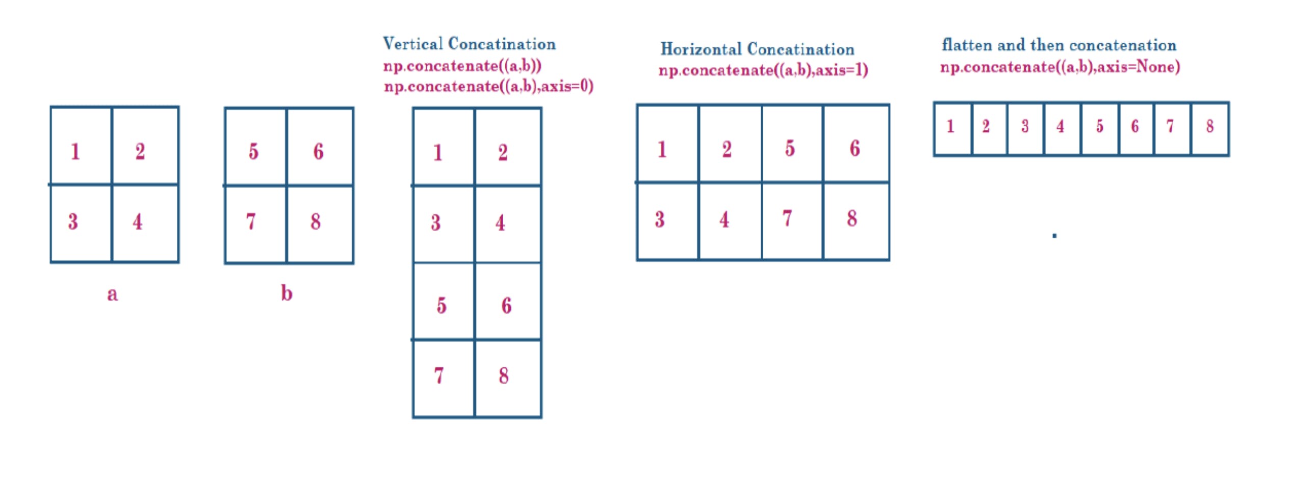
concatenate()
This function is used to join arrays along an axis.
Rule of concatenation -
We can join any number of arrays, but all arrays should be of the same dimension.
The sizes of all axes, except the concatenation axis, should be the same.
The shapes of the resultant array and out array must be the same.
concatenate((a1, a2, ...), axis=0, out=None, dtype=None, casting="same_kind")

#a1, a2, ... : arrays you want concatenate
#axis : The axis along which the arrays will be joined. Can be 0, 1 or None
#out : the destination to place the result. The shape must match.
Examples of concatenate() -
#1D array
a = np.arange(4)
b = np.arange(5)
c = np.arange(3)
np.concatenate((a,b,c))
#output - array([0, 1, 2, 3, 0, 1, 2, 3, 4, 0, 1, 2])

#2D array
a = np.array([[1,2],[3,4]])
b = np.array([[5,6],[7,8]])
# concatenation by providing axis paraameter
# Vertical Concatenation
vcon = np.concatenate((a,b))
vcon1 = np.concatenate((a,b),axis=0)
# Horizontal Concatenation
hcon = np.concatenate((a,b),axis=1)
# flatten and then concatenation
flatt = np.concatenate((a,b),axis=None)
print(f"array a ==> \n {a}")
print(f"array b ==> \n {b}")
print(f"Without specifying axis parameter ==> \n {vcon}")
print(f"Specifying axis=0 a ==> \n {vcon1}")
print(f"Specifying axis=1 ==> \n {hcon}")
print(f"Specifying axis=None ==> \n {flatt}")
#output - array a ==>
#[[1 2]
#[3 4]]
#array b ==>
#[[5 6]
#[7 8]]
#Without specifying axis parameter ==>
#[[1 2]
#[3 4]
#[5 6]
#[7 8]]
#Specifying axis=0 a ==>
#[[1 2]
#[3 4]
#[5 6]
#[7 8]]
#Specifying axis=1 ==>
#[[1 2 5 6]
#[3 4 7 8]]
#Specifying axis=None ==>
#[1 2 3 4 5 6 7 8]
stack()
Used to join multiple arrays along a new axis. The joining arrays must have the same shape and size. If we stack two 1D arrays we get a 2D array as a result. Similarly, if we stack two 2D arrays we get a 3D array as result. We can stack arrays about any of the axes.
numpy.stack(arrays, axis=0, out=None, *, dtype=None, casting='same_kind')
Examples -
# stacking using axis=0
a = np.array([10,20,30])
b = np.array([40,50,60])
resultant_array = np.stack((a,b)) # default axis=0
print(f"Resultant array : \n {resultant_array}")
print(f"Resultant array shape: {resultant_array.shape}")

#output - Resultant array :
#[[10 20 30]
#[40 50 60]]
#Resultant array shape: (2, 3)

# stacking using axis=1
a = np.array([10,20,30])
b = np.array([40,50,60])
resultant_array=np.stack((a,b),axis=1)
print(f"Resultant array : \n {resultant_array}")
print(f"Resultant array shape: {resultant_array.shape}")
#output - Resultant array :
#[[10 40]
#[20 50]
#[30 60]]
#Resultant array shape: (3, 2)
vstack()
Used for stacking arrays vertically(row-wise). Same as concatenate() along axis 0. If we stack two 1D arrays , we get 2D array as an output.
numpy.vstack(tup, *, dtype=None, casting='same_kind')

#tup : sequence of ndarray
Examples showing how to use vsatck() -
#1D array
# vstack for 1-D arrays of same sizes
a = np.array([10,20,30,40])
b = np.array([50,60,70,80])
# a will be converted to shapes (1,4) and b will be converted to (1,4)
np.vstack((a,b))
#output - array([[10, 20, 30, 40],
#                [50, 60, 70, 80]])

a = np.arange(1,10).reshape(3,3)
b = np.arange(10,16).reshape(2,3)
np.vstack((a,b))
#output - array([[ 1, 2, 3],
#                [ 4, 5, 6],
#                [ 7, 8, 9],
#                [10, 11, 12],
#                [13, 14, 15]])
hstack()
Stack arrays in sequence horizontally (column wise). This is equivalent to concatenation along the second axis, except for 1-D arrays where it concatenates along the first axis.
numpy.hstack(tup, *, dtype=None, casting='same_kind')
#For 1-D arrays
a = np.array([10,20,30,40])
b = np.array([50,60,70,80,90,100])
np.hstack((a,b))
#output - array([ 10, 20, 30, 40, 50, 60, 70, 80, 90, 100])

#For 2-D arrays
a = np.arange(1,7).reshape(3,2)
b = np.arange(7,16).reshape(3,3)
np.hstack((a,b))
#output - array([[ 1, 2, 7, 8, 9],
#                [ 3, 4, 10, 11, 12],
#                [ 5, 6, 13, 14, 15]])
dsplit()
Used to stack arrays in sequence depth-wise (along third axis). This is equivalent to concatenation along the third axis after 2-D arrays of shape (M,N) have been reshaped to (M,N,1) and 1-D arrays of shape (N,) have been reshaped to (1,N,1).
a = np.array([1,2,3])
b = np.array([2,3,4])
np.dstack((a,b))
#output - array([[[1, 2],
#                 [2, 3],
#                 [3, 4]]])
Splitting Arrays
split()
Split an array into multiple sub-arrays of equal size. It returns list of ndarray objects.
split(array, indices_or_sections, axis=0)
#array : Array to be divided into sub-arrays.
#indices_or_sections : If indices_or_sections is an integer, N, the array will be divided into N equal arrays along axis. If such a split is not possible, an error is raised.
Some examples of its use -
a = np.arange(1,10)
sub_arrays = np.split(a,3)
print(f"array a : {a}")
print(f"Type of sub_arrays :{type(sub_arrays)}")
print(f"sub_arrays : {sub_arrays}")

#output - array a : [1 2 3 4 5 6 7 8 9]
#Type of sub_arrays :<class 'list'>
#sub_arrays : [array([1, 2, 3]), array([4, 5, 6]), array([7, 8, 9])]

# split based on default axis i.e., axis-0 (Vertical Split)
a = np.arange(1,25).reshape(6,4)
result_3sections = np.split(a,3) # dividing 3 sections vertically
print(f"array a : \n {a}")
print(f"splitting the array into 3 sections along axis-0 : \n {result_3sections}")
# Note: Here we can use various possible sections: 2,3,6

#output - array a :
#[[ 1 2 3 4]
#[ 5 6 7 8]
#[ 9 10 11 12]
#[13 14 15 16]
#[17 18 19 20]
#[21 22 23 24]]
#splitting the array into 3 sections along axis-0 :
#[array([[1, 2, 3, 4],
# [5, 6, 7, 8]]), array([[ 9, 10, 11, 12],
# [13, 14, 15, 16]]), array([[17, 18, 19, 20],
# [21, 22, 23, 24]])]

# splitting the 1-D array based on indices
a = np.arange(10,101,10)
result = np.split(a,[2,5,7])
# [2,5,7] ==> 4 subarrays
# subarray-1 : before index-2 ==> 0,1
# subarray-2 : from index-2 to before index-5 ==> 2,3,4
# subarray-3 : from index-5 to before index-7 ==> 5,6
# subarray-4 : from index-7 to last index ==> 7,8,9
print(f"array a : {a}")
print(f"splitting the 1-D array based on indices : \n {result}")

#output - array a : [ 10 20 30 40 50 60 70 80 90 100]
#splitting the 1-D array based on indices :
#[array([10, 20]), array([30, 40, 50]), array([60, 70]), array([ 80, #90, 100])]
Sorting an Array
sort()
Returns a sorted version of the array without modifying the values.
x = np.array([2, 1, 4, 3, 5])
np.sort(x)
#output - array([1, 2, 3, 4, 5])

#If you prefer to sort the array in-place, you can instead use the sort method of arrays:
x.sort()
print(x)
#output - [1 2 3 4 5]

#Sorting along a column
# sort each column of X
X = np.random.randint(0, 10, (4, 6))
np.sort(X, axis=0)
#output - [[2 7 4 6 6 0]
#          [9 2 4 5 4 6]
#          [4 0 3 4 4 9]
#          [4 6 5 1 6 3]]
argsort()
Return the indices of the elements of the sorted array.
x = np.array([2, 1, 4, 3, 5])
i = np.argsort(x)
print(i)
#output - [1 0 3 2 4]
Conclusion
This ends our blog on NumPy in detail. However, some concepts such as Broadcasting are still left because the purpose of this blog was to get you comfortable with numpy and its various function. This is supposed to be a beginner's guide to numpy and if you completed it, I would recommend you to learn more by practising it. Being comfortable with numpy will help you while studying other libraries like pandas and matplotlib. Thanks for reading this blog, I hope this blog helped you.