

Photo by Louis Hoang on Unsplash
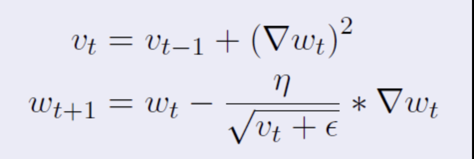
AdaGrad Algorithm
Understanding Adagrad Optimization Algorithm and writing simple Python code to implement and visualize it.


What is Adagrad?
Short for Adaptive Gradient Algorithm, Adagrad is an optimization algorithm designed to adaptively adjust the learning rate for individual parameters. The key idea is to give a small learning rate to parameters with a large gradient and a larger learning rate to parameters with a small gradient in the past. This adaptive scaling aims to make the optimization process more efficient by allowing for larger updates for less frequently occurring features and smaller updates for more frequently occurring ones.
Adagrad Algorithm
- Initialize Parameters:
Initialize the parameter vector θ: θ←initialize_theta()
Initialize the vector G to keep track of the accumulated squared gradients: G←initialize_accumulated_gradient()
- Set Hyperparameters:
Set the value of ϵ (a small constant to avoid division by zero): ϵ←set_epsilon_value()
Set the value of the learning rate (η): η←set_learning_rate()
- Until termination criteria are met, do:
For each iteration t:
Sample a minibatch of training examples: minibatch←sample_minibatch(training_data)
Compute the gradient of the cost function with respect to the parameters: ∇J(θ)←compute_gradient(cost_function,θ, minibatch)
Update the accumulated squared gradient: G←G+(∇J(θ))^2
Update the parameters using the Adagrad update rule: θ←θ−G+ϵη⋅∇J(θ)
Implementation
We are going to write create an AdagradOptimizer class to implement the above algorithm
import numpy as np

class AdagradOptimizer:
    def __init__(self, learning_rate=0.01, epsilon=1e-8):
        self.learning_rate = learning_rate
        self.epsilon = epsilon
        self.gradient_accumulator = None

    def update(self, params, gradients):
        if self.gradient_accumulator is None:
            self.gradient_accumulator = np.zeros_like(params)

        # Update the accumulated squared gradients
        self.gradient_accumulator += gradients ** 2

        # Compute the adaptive learning rate
        adaptive_learning_rate = self.learning_rate / (np.sqrt(self.gradient_accumulator) + self.epsilon)

        # Update the model parameters
        params -= adaptive_learning_rate * gradients

        return params
To check the above class we do the following:
# Example usage:
# Initialize model parameters and gradients
params = np.random.rand(5)
gradients = np.random.rand(5)

# Create an Adagrad optimizer
optimizer = AdagradOptimizer(learning_rate=0.01)

# Update parameters using Adagrad
updated_params = optimizer.update(params, gradients)

# Print the updated parameters
print("Original Parameters:", params)
print("Updated Parameters:", updated_params)

# Output -
Original Parameters: [0.14287995 0.49640699 0.27355323 0.24208914 0.80852391]
Updated Parameters: [0.14287995 0.49640699 0.27355323 0.24208914 0.80852391]
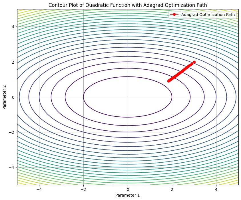
Visualizing
We will create a contour plot to visualize the working of Adagrad algorithm and how it reaches the minima.
import numpy as np
import matplotlib.pyplot as plt

# Define the quadratic function
def quadratic_function(x, y):
    return x**2 + 3 * y**2

# Create a meshgrid for the contour plot
x = np.linspace(-5, 5, 100)
y = np.linspace(-5, 5, 100)
X, Y = np.meshgrid(x, y)
Z = quadratic_function(X, Y)

# Initialize Adagrad optimizer
optimizer = AdagradOptimizer(learning_rate=0.1)

# Number of iterations
num_iterations = 50

# Initial parameters
params = np.array([3.0, 2.0])

# Lists to store parameter values during optimization
param_history = [params.copy()]

# Perform optimization
for _ in range(num_iterations):
    gradients = np.array([2 * params[0], 6 * params[1]])  # Gradient of the quadratic function
    params = optimizer.update(params, gradients)
    param_history.append(params.copy())

# Create contour plot
plt.figure(figsize=(10, 8))
plt.contour(X, Y, Z, levels=30, cmap='viridis')
param_history = np.array(param_history)
plt.plot(param_history[:, 0], param_history[:, 1], marker='o', color='red', label='Adagrad Optimization Path')
plt.title('Contour Plot of Quadratic Function with Adagrad Optimization Path')
plt.xlabel('Parameter 1')
plt.ylabel('Parameter 2')
plt.legend()
plt.grid(True)
plt.show()
Drawbacks
See how in the graph, the red line stops before reaching the centre of the graph. That is one of the major drawbacks of Adagrad.
The accumulation of squared gradients in the denominator can lead to a very small learning rate over time. This can cause learning to stop. Adagrad does not include momentum, which is a term that helps accelerate optimization by dampening oscillations and speeding up convergence. More recent optimization algorithms like RMSprop and Adam address this limitation by incorporating momentum-like terms.
Conclusion
This article was about the simple implementation of Adagrad optimization algorithm and visualizing it using a contour plot. This information here alone is not enough to get a detailed understanding of adaptive optimization algorithms. I would advise you to study more on this topic to understand this in depth. Feel free to ask any questions. Thanks for reading.